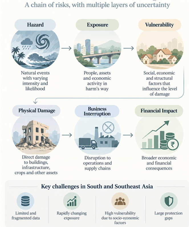
1. A disaster can cut the value of an asset even if the asset itself stays whole.
In December 2023, Cyclone Michaung brought intense rainfall and widespread flooding to Tamil Nadu, particularly Chennai and the surrounding districts. The event disrupted transport, power, businesses and essential services across the affected areas. A World Bank assessment estimated that Cyclone Michaung and the subsequent floods resulted in ₹15,645 crore in total economic losses, including ₹4,966 crore in direct damage and ₹10,679 crore in indirect losses. The scale of indirect losses illustrates that the financial consequences of a catastrophe can extend far beyond the physical assets directly damaged by the event.
The distinction is important because disaster losses extend beyond the assets directly damaged by the hazard and can propagate through businesses, infrastructure, supply chains and the wider economy. UNDRR’s Global Assessment Report 2025 estimates that while direct disaster losses are reported at more than US$200 billion annually, the total cost rises to more than US$2.3 trillion a year when cascading and ecosystem-related impacts are considered.
This is what makes financial-loss modelling different from simply mapping a hazard. A flood map can show where water may reach, but a financial-loss model must establish what is exposed, how those assets respond to the hazard, what gets damaged, how long economic activity is disrupted and how those impacts translate into financial consequences. In UNDRR’s risk framework, disaster risk is shaped by the interaction of hazard, exposure and vulnerability, while the resulting losses can take different forms and are often difficult to quantify.
For South and Southeast Asia, the critical question is no longer simply where a catastrophe may occur.
It is:
What happens after the hazard strikes and how much does it really cost?
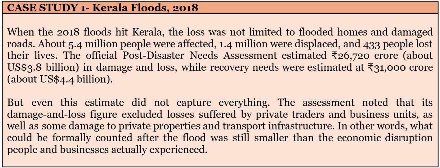
SOURCE- UNDP
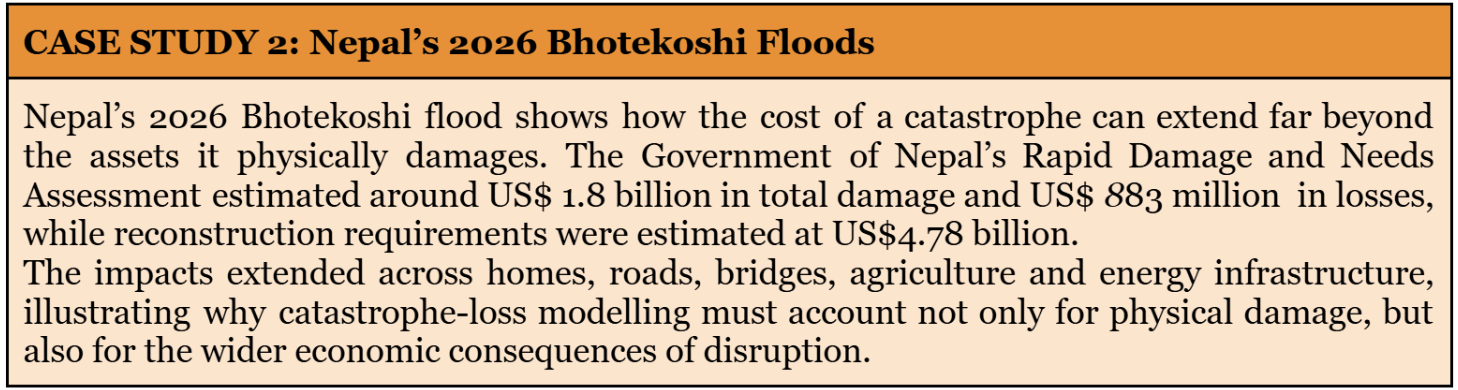
Source: Ministry of foreign affairs
These cases point to a broader problem: the difficulty is not simply identifying that a disaster occurred, but measuring how its effects propagate across assets, sectors and the wider economy.
2. Why South and Southeast Asia Are Particularly Difficult to Model?
The challenge of catastrophe-loss modelling in South and Southeast Asia is not merely the frequency of floods, cyclones and other natural hazards. It is the difficulty of translating a changing physical environment into a reliable financial estimate. In this region, this is tough for one main reason. The data needed for the estimate does not stay the same over time, and it does not sit nicely in one source.
Cities are growing and people and assets are shifting into new areas. At the same time, hazard and loss observations differ a lot from place to place. Research across mainland Southeast Asia shows how quickly this can alter future exposure. Tierolf et al. (2021) found that projected urban development increased expected annual flood damage in Cambodia, Laos, Myanmar, Thailand and Vietnam, with increases ranging from 8% in Thailand to 211% in Laos.
Figure 1 : Projected Increase in Expected Annual Flood Damage by 2040
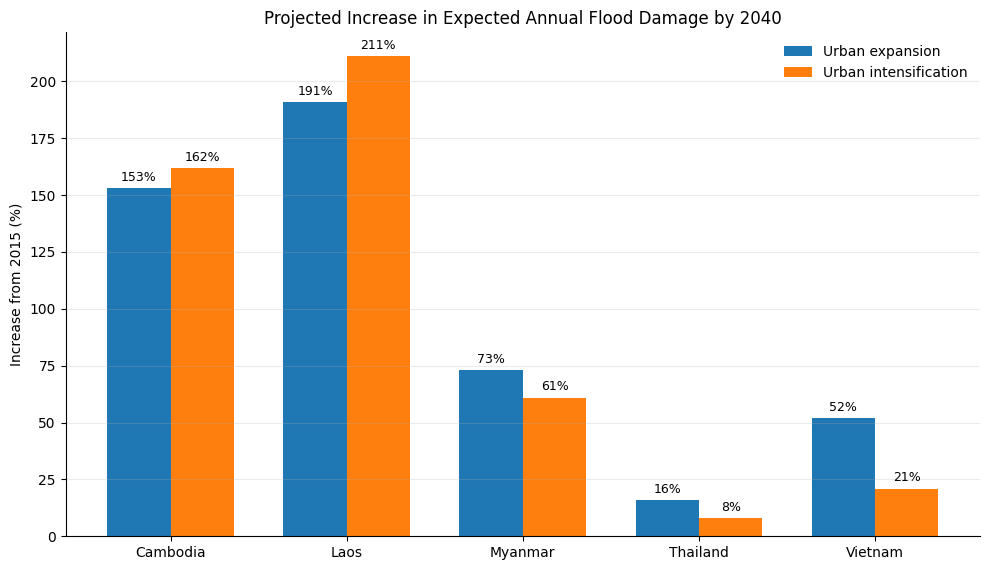
SOURCE: Projected increase in expected annual flood damage by 2040 under alternative urban-development scenarios in mainland Southeast Asia. Adapted from Tierolf et al. (2021).
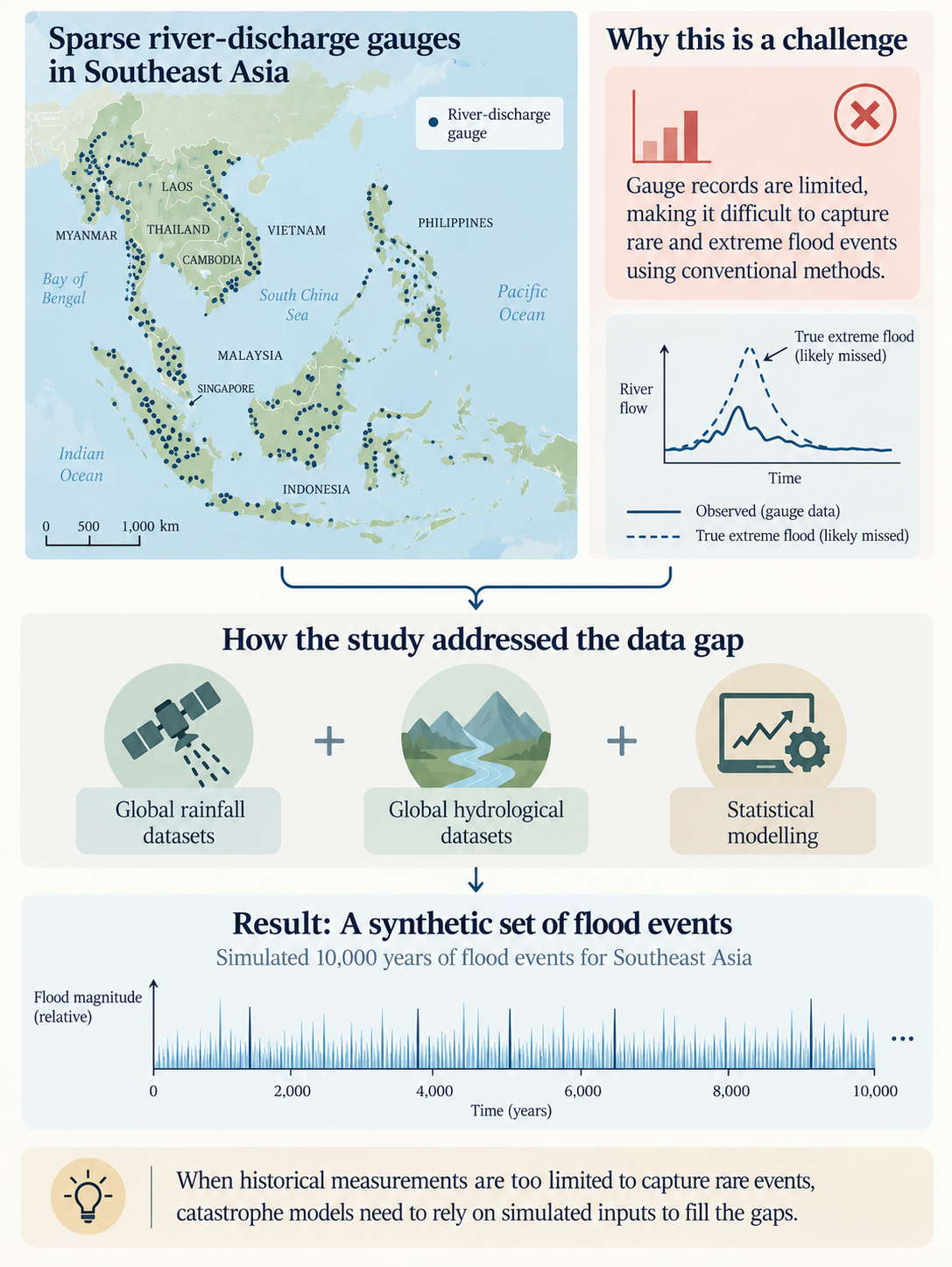
But knowing where exposure is changing is only one part of the problem. The hazard itself may also be difficult to characterise, particularly when historical observations are sparse.Olcese et al. (2024), for example, identified only around 300 river-discharge gauges across 4.5 million km² of Southeast Asia—equivalent to roughly one gauge per 15,000 km². By comparison, the United States has more than 11,000 gauges across 9.4 million km², or approximately one gauge per 855 km², highlighting the much greater observational density available in a data-rich economy.
For catastrophe modelling, the implication is important: limited observations make it difficult to represent rare and extreme floods from historical records alone. Olcese et al. therefore combined global rainfall and hydrological datasets with statistical modelling to generate a synthetic flood catalogue representing 10,000 years. The approach illustrates a broader challenge: where historical observations cannot capture the full range of possible events, models must reconstruct the missing tail of the risk distribution.
Figure 2: Synthetic Flood Events for Extreme Flood Risk Modelling Beyond the Historical Record
Note: Image is for representation purpose only.
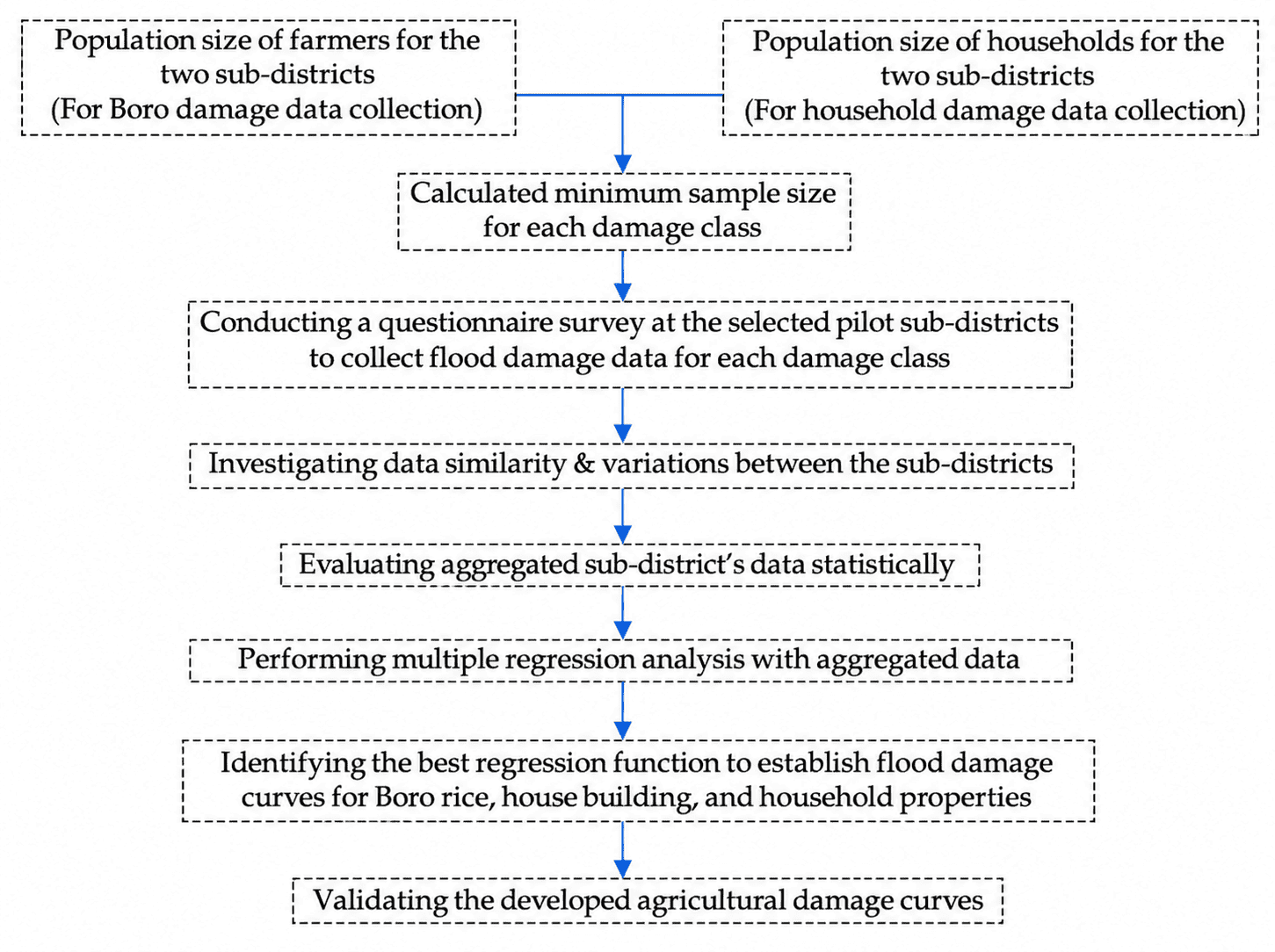
The uncertainty does not end once the hazard has been modelled. The next question is how that hazard translates into physical damage. In Bangladesh, researchers in paper (Khairul et al., 2022) found that actual flood-damage records were limited, inconsistent and fragmented, requiring synthetic flood-damage functions developed from questionnaire survey data. Their results differed across construction types, demonstrating how difficult it is to apply a single vulnerability assumption across different assets.
Figure 3. Methodology used by Khairul et al. (2022) to develop synthetic flood-damage functions from questionnaire survey data.
SOURCE:Khairul et al. (2022)
Taken together, these studies show that the problem is not simply a lack of data, but a lack of consistent data across the modelling chain. Exposure is changing, hazard observations are sparse, and the relationship between hazard intensity and physical damage is not always well documented. The challenge is therefore to connect hazard, exposure and vulnerability well enough to estimate how an event ultimately translates into economic and financial loss.
3. Challenge 1 — Determining Exposure: What Is Actually There?
In catastrophe modelling, exposure is the layer that converts a hazard footprint into something with economic meaning. It is not enough to know that a flood, cyclone or earthquake passes through a particular area. The model must identify which assets are located there, what those assets are, how they are constructed, and what value or economic activity they represent. These attributes perform two different functions: location determines the hazard intensity assigned to an asset, while characteristics such as occupancy, construction and year built help determine the appropriate vulnerability relationship. The financial value attached to that exposure then determines how physical damage is translated into monetary loss.
The difficulty across the region is that this information is often fragmented rather than absent altogether.
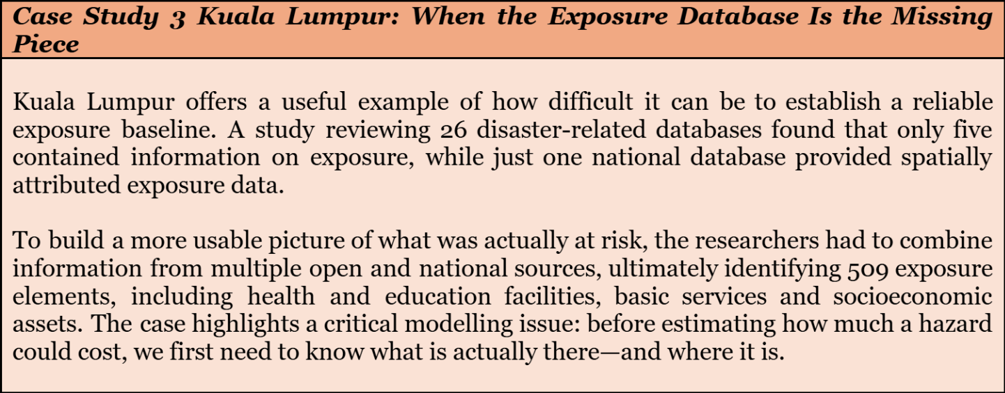
But identifying where an asset is located is only the first step. To estimate its potential loss, the model must also know what the asset is, how it is used, how it is constructed and what it is worth. Details such as occupancy, construction type and year built influence which vulnerability function is applied, while the choice of insured or replacement value affects the resulting monetary loss. If exposure data are outdated or incomplete, these uncertainties can carry through to the final loss estimate.
Exposure is also dynamic rather than fixed. In the Philippines, Johnson et al. (2021) estimated that 6,040–13,850 hectares of urban land could be converted in flood-prone areas between 2019 and 2050, potentially affecting 2.5–5.8 million additional residents.
Figure 4: Expanding cities, growing exposure
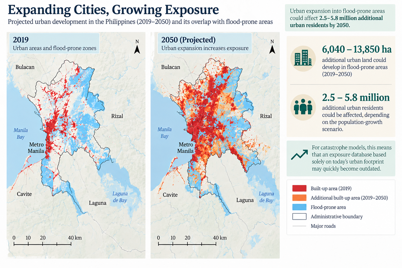
SOURCE: Projected expansion of urban development into flood-prone areas in the Philippines, 2019–2050. Adapted from Johnson et al. (2021).
These limitations compound through the loss model: a missing asset cannot be valued, a mislocated asset may receive the wrong hazard intensity, and a poorly classified or valued asset may be assigned an inappropriate damage estimate. UNDRR therefore emphasises georeferenced, disaggregated and sector-specific exposure data, including inventories of assets and production systems beyond basic building and population counts.
4. Challenge 2 — Determining the Hazard: How Intense Is the Event at the Asset?
For financial-loss modelling, knowing that an asset is located in a hazard-prone area is not enough. Hazard probability and hazard intensity are different measures: probability describes how often an event of a particular severity may occur, while intensity describes what the asset actually experiences. Catastrophe models therefore represent events through their frequency and spatial footprint, together with intensity measures such as flood depth, velocity and duration, wind speed, rainfall, storm surge or ground shaking.
The temporal dimension is equally important. A flood reaching the same depth can produce very different damage depending on how long the water remains. Research from Bangladesh’s Teesta River Basin, for example, found that residential flood damage is influenced not only by depth but also by flood duration and velocity, showing why a single depth–damage relationship may not adequately represent actual impacts.
Figure 5: Illustration of how flood duration and velocity can influence damage at the same flood depth.
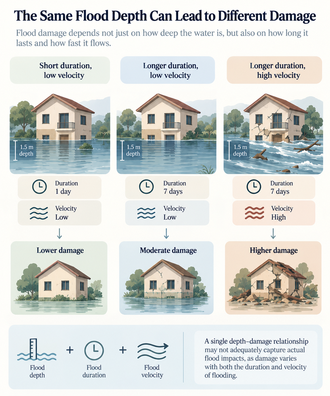
Note: Image is for representation purpose only.
When Hazards Occur Together
Hazard uncertainty also becomes more complex when multiple hazards occur together. A tropical cyclone can bring extreme wind, rainfall and storm surge, followed by inland flooding; one hazard can therefore intensify the consequences of another. Ranjan and Karmakar (2024), analysing cyclone events across India from 1979–2020, found substantial spatial variation in the frequency and duration of concurrent extreme wind and rainfall. In parts of eastern India, such concurrent extremes could persist for more than 24 hours, demonstrating why cyclone severity cannot always be represented by peak wind speed alone.
Slow-Onset Hazards
The current 2026–27 El Niño is developing as an unusually strong event, driven by exceptionally warm sea-surface temperatures across the equatorial Pacific. NOAA reports sea-surface temperature anomalies exceeding 3°C in the eastern equatorial Pacific, with a greater than 90% chance of a very strong event during late 2026 and winter 2026–27. Current forecasts indicate that El Niño conditions may persist into spring 2027, extending the period over which associated heat, rainfall and drought risks can be felt across different parts of the world.
For financial-loss modelling, heat presents a different challenge from a flood or cyclone because its impacts accumulate gradually and are often dispersed across the economy. Crop yields may fall, heat-related mortality may rise, labour productivity may decline and wages may be lost, while electricity demand increases, putting pressure on grids and increasing the risk of power and equipment failures. These effects can ultimately translate into infrastructure damage, higher operating costs and substantial economic losses, yet many remain difficult to identify and quantify because they occur across multiple sectors rather than as a single recorded event.
Figure 6: How extreme heat translates into economic losses
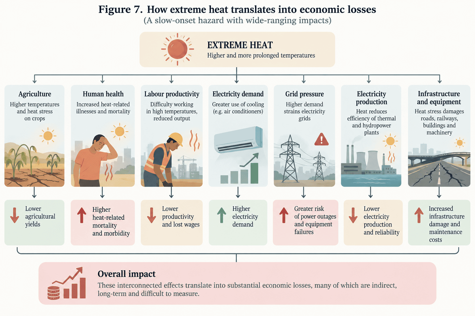
Note: Image is for representation purpose only.
UNDRR’s GAR 2025 reports that multi-hazard events represented around 19% of recorded disasters but almost 59% of economic losses in its analysis. The modelling challenge is therefore to capture not just whether a hazard occurs, but its intensity, duration, spatial footprint and interaction with other hazards.
5. Challenge 3 — Vulnerability: How Much Damage Does a Given Hazard Cause?
The same hazard does not produce the same damage everywhere. A one-metre flood, for example, can affect buildings very differently depending on their construction, elevation, use and contents. Vulnerability functions capture this relationship by linking hazard intensity to an expected damage ratio for a particular asset type. Their reliability is therefore central to converting hazard information into a credible loss estimate. (Déroche, 2023)
The difficulty is that reliable vulnerability functions require observed damage data matched with hazard intensity and asset characteristics—data that remain limited in many South and Southeast Asian markets. In Bangladesh’s Meghna Basin, Khairul et al. (2022) developed flood-damage functions from surveys of 165 households, covering mud, brick and concrete houses. The study found clear differences between construction types: mud houses were the most vulnerable, with damage reaching total levels when floodwater exceeded 150 cm above the plinth, while brick and concrete houses generally remained partially damaged.
Figure 7. Developed flood-damage curves for mud, brick and concrete houses, illustrating differences in vulnerability across construction types.
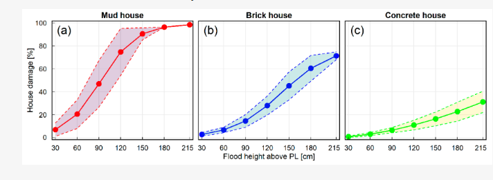
Source: the flood-damage curves for mud, brick and concrete houses.
Vulnerability also extends beyond the structure itself. Physical characteristics influence direct damage, while operational conditions—such as access, utilities and backup systems—affect whether an asset can continue functioning. Social and economic conditions, including income, access to finance and institutional support, further shape how people and businesses absorb and recover from a disaster. (World Bank)
The model then translates this vulnerability into physical damage to buildings, machinery, inventory and infrastructure, usually by applying a damage ratio to the relevant asset value or replacement cost. The challenge is that uncertainty in the vulnerability function, asset characteristics or valuation can all carry through to the final financial estimate.
In essence, the modelling problem is not simply predicting how intense the hazard will be, but determining how different assets will respond to it—and how that response translates into monetary damage.
6. Business Interruption: The Hidden Component of Catastrophe Loss
When Physical Damage Is Only Part of the Loss
Physical damage tells us what a catastrophe destroys; business interruption (BI) captures what happens when economic activity cannot continue normally. A business may suffer relatively limited physical damage yet face substantial losses if production, access to utilities, transport or supplies remains disrupted. The duration of the interruption, recovery time, dependence on infrastructure, supply-chain connections and the firm’s ability to shift production or find alternatives can therefore be as important as the damage to the asset itself.
Evidence from South Asia shows why this distinction matters. The World Bank’s From Risk to Resilience study found that, across weather shocks reported by surveyed firms over the past five years (2019–24), declining sales accounted for 46% of reported damages, compared with 9% from repairing or replacing damaged physical assets. For firms experiencing flooding or sea-level rise, the average event cost was around 6% of annual revenue.
Figure 8: Damages to firm operation from weather shocks,2019–24
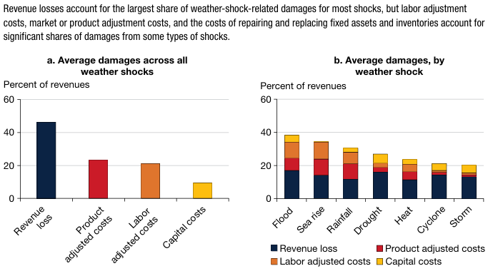
Source: The World Bank’s From Risk to Resilience study
Disruption Spreads Beyond the Affected Business
BI can also spread beyond the directly affected business. A direct loss occurs when the firm’s own premises or operations are disrupted; an indirect loss can arise when a supplier or customer is affected; and a systemic disruption can occur when failure of critical infrastructure, such as electricity, interrupts multiple businesses simultaneously. Indian evidence provides another illustration. Goldar et al. (2025), found that cyclones were followed by a 4–6% decline in sales and a 2–3% decline in total assets among manufacturing firms, with larger sales effects among smaller firms.
For catastrophe modelling, the challenge is therefore to estimate not only how long business activity is disrupted, but how that disruption propagates through infrastructure and supply chains.
7. From Economic Loss to Financial Loss: The Protection Gap
A catastrophe can generate substantial economic losses without creating an equivalent insured loss. Physical damage, wider economic loss and insured loss are different measures: a damaged factory may incur repair costs, lost production and disrupted cash flows, while only part of those losses may be covered by insurance. In emerging and developing Asia-Pacific, OECD estimates that only 5–7% of natural-hazard losses were insured between 2000 and 2023, illustrating the scale of the protection gap.
Figure 9. Estimated share of natural-hazard economic losses covered by insurance across selected Asian economies, 2000–2023.
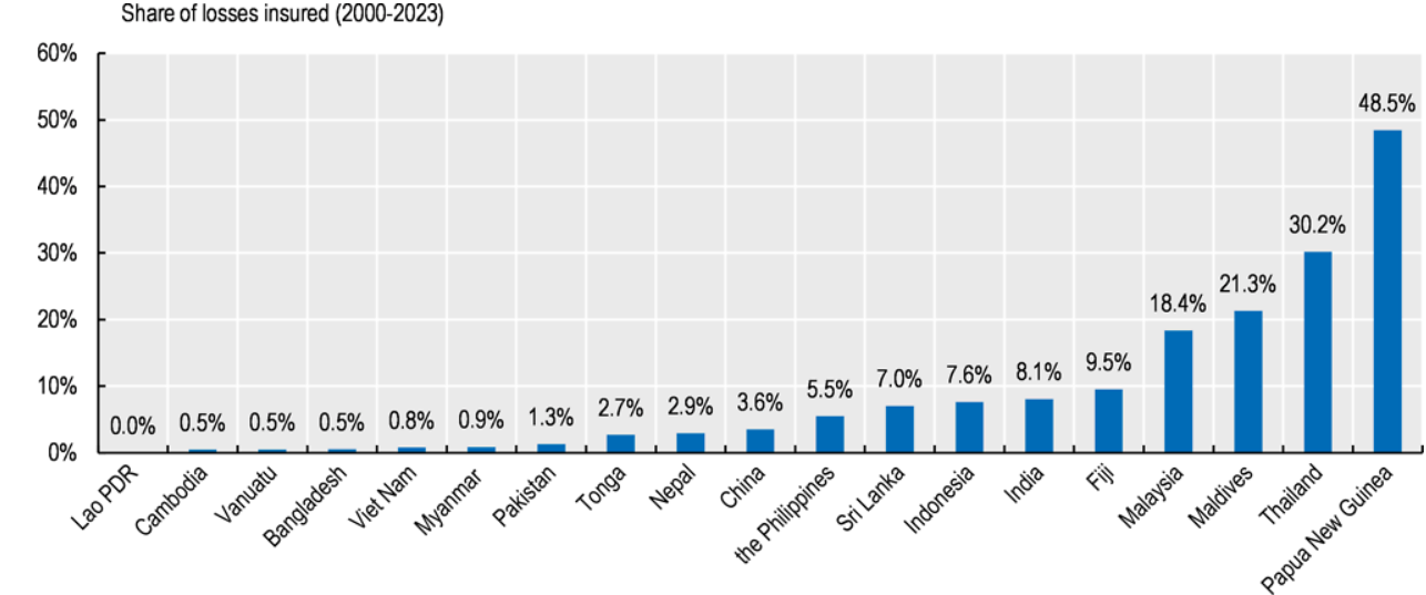
Source: OECD, Protection Gaps in Insurance for Natural Hazards and Retirement Savings in Asia (2025).
The problem is compounded by the missing-loss-data problem. Damage to buildings and infrastructure is generally easier to record than the associated loss of services, production or income. UNDRR’s review of 57 Post Disaster Needs Assessments found that infrastructure losses and service disruptions were reported less frequently than physical damage, citing limited pre-disaster data and difficulties in estimating service disruption.
This creates a difficult environment for financial-loss modelling. Limited claims and loss histories provide less evidence for calibrating risk, while OECD notes that inadequate data and catastrophe-risk assessment tools can constrain insurers’ ability to quantify and price natural-hazard losses.
The final question is therefore who ultimately bears the loss. An insurer may face claims; a bank may face weakened collateral and borrower cash flows; a business may absorb uninsured repair costs and revenue losses; and governments may face reconstruction and fiscal pressures. The protection gap is therefore not simply an insurance problem—it determines how catastrophe losses are distributed across the wider financial system.
8. Building Better Financial-Loss Models Under Data Constraints
Combining Imperfect Data
Better financial-loss modelling in South and Southeast Asia does not necessarily require a perfect dataset. It requires combining the best available evidence and making uncertainty explicit. Adaptation should be part of this process: two otherwise similar assets may experience different losses because one has elevated machinery, flood protection, backup power or alternative suppliers. The World Bank finds that firms across South Asia are already taking adaptation measures, although most remain relatively basic, highlighting the importance of incorporating resilience into risk assessment rather than treating it as an afterthought.
Where direct loss data are limited, models can combine several layers of information: observed claims and damage assessments, engineering vulnerability functions, remote-sensing data and socioeconomic or economic proxies, supplemented by expert judgement where necessary. The objective is not to conceal gaps in the evidence, but to understand how those gaps affect the resulting loss estimate.
Quantifying the Probability of Loss
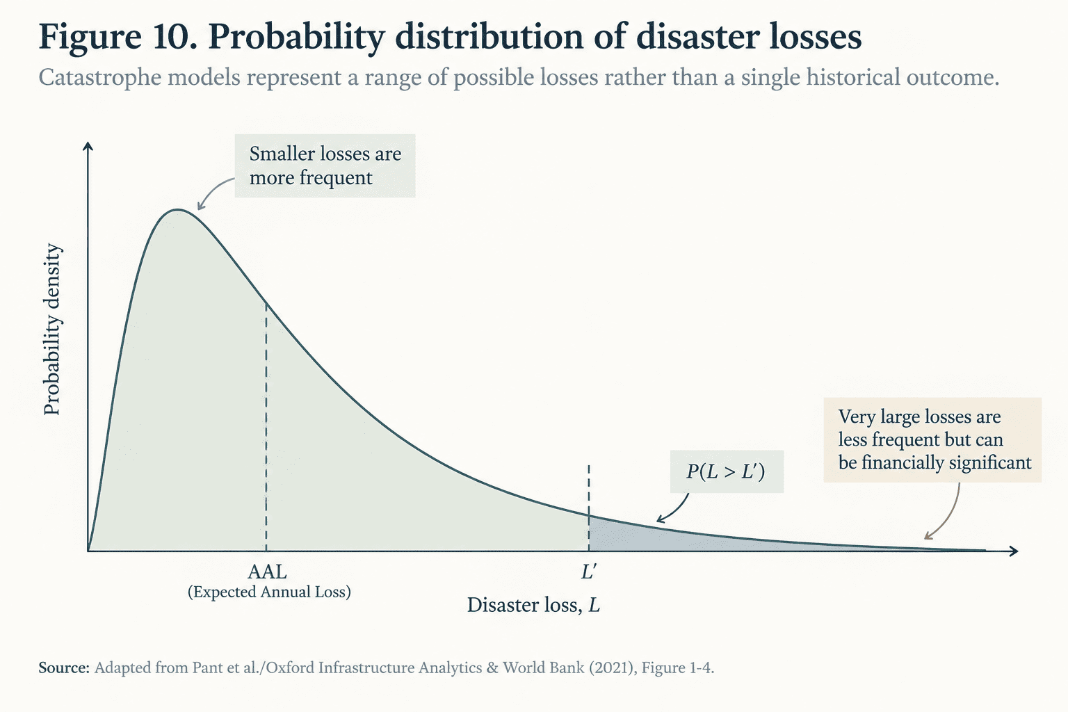
A probabilistic approach is more useful than relying on a single historical event. Instead of asking what the next cyclone or flood will cost, catastrophe models can estimate a distribution of possible losses, including Expected Annual Loss and losses associated with different return periods. GAR 2025 emphasises the importance of robust risk information and metrics such as annual average losses and probable maximum losses for financial decision-making.
One way of expressing this uncertainty is through a loss-probability curve, which shows how the estimated size of a loss changes as the probability of that loss changes. Lower-probability events represent rarer and generally more severe outcomes, while higher-probability events represent more frequent, lower-loss outcomes.
Figure 10. Probability distribution of disaster losses, illustrating Expected Annual Loss (AAL) and the probability that losses exceed a specified level (L′).
SOURCE: Pant et al./Oxford Infrastructure Analytics & World Bank (2021)
A practical modelling framework should connect exposure and probabilistic hazard estimates with locally appropriate vulnerability functions, and then trace their effects through physical damage, business interruption, insurance and wider financial consequences. At each stage, uncertainty in the underlying data and assumptions should be carried forward rather than overlooked. The goal is not to predict a single outcome with certainty, but to produce a transparent and credible range of potential financial losses.
9. Conclusion – The Objective Isn’t Perfect Prediction
The challenge in across the region is not simply identifying where natural hazards may occur. The harder task is translating those hazards into physical damage, business interruption, economic loss and, ultimately, financial consequences in markets where exposure is changing, vulnerability data are uneven and protection gaps remain substantial.
A reliable estimate will therefore rarely come from a single dataset or model. It requires bringing together hazard science, exposure information, vulnerability functions, socioeconomic conditions, event-loss data and financial information, while making the uncertainty in each component visible rather than hiding it.
The objective is not perfect prediction. It is to build models that provide a transparent and credible range of potential losses, allowing insurers, businesses, banks and policymakers to understand not only where risk lies, but how a catastrophe can translate into financial impact.
The next generation of catastrophe modelling must therefore move from mapping hazards to quantifying consequences.
FIGURE 11: How natural hazard translates into financial impact.